Measurement Error
Henry Lu,
Sylvia Li
Reliability Theory
Reliability refers to the consistency of a test or
measurement. It shows the reproducibility of same test results in repeated
trials. Better reliability implies higher precision of single measurement, as
well as better tracking of changes in measurements in research or practical
settings.
Reliability consists of absolute and relative consistency.
Absolute consistency indicates the consistency of scores of individuals,
whereas relative consistency concerns the consistency of the position or rank
of individuals in the group relative to others.
Relative consistency is quantified through intraclass
correlation coefficient (ICC). Absolute consistency is quantified by standard
error of measurement (SEM) or variations such as minimum detectable difference
(MDD) and standard error of prediction (SEP).
Observed and true
scores
The observed score is the number of points obtained on the
test. Each observed score includes two parts, the true score, which is the mean
of an infinite number of scores from the individual (ppt), and the error score,
which is the difference between the observed score and true score.
Reliability
coefficient
For a group of measurements, the total variance (![]() ) in
the data is composed of true score variance (
) in
the data is composed of true score variance (![]() ) and
error variance (
) and
error variance (![]() ), which
can be expressed as:
), which
can be expressed as:
![]()
The reliability coefficient is defined as:
![]()
The closer the reliability coefficient is to 1.0, the
higher the reliability and the lower the ![]() .
.
Since the true score of each subject is not actually known,
![]() is used based on the between-subjects
variability, i.e., the variance due to how subjects differ from each other.
Thus, the formal definition of reliability coefficient becomes:
is used based on the between-subjects
variability, i.e., the variance due to how subjects differ from each other.
Thus, the formal definition of reliability coefficient becomes:
![]()
The reliability coefficient could be quantified by various
ICCs.
Intraclass Correlation Coefficient (ICC)
Definition
ICC is a relative measure of reliability in that it is a
ratio of variances derived from ANOVA, which represents the proportion of
variance in a set of scores that is attributable to ![]() .
.
Interpretation
and properties
An ICC of 0.95 means that an estimated 95% of the observed
score variance is due to the true score variance ![]() , and
that an estimated 5% of the observed score variance is due to the error
variance
, and
that an estimated 5% of the observed score variance is due to the error
variance ![]() .
.
The magnitude of ICC depends on the between-subject
variability, that ICC values are small when subjects differ little from each
other, and vice versa.
ICC is unitless and theoretically varies between 0 and 1.
ICC of 0 indicates no reliability, while ICC of 1 implies perfect reliability.
Choices of
ICC models
To calculate the ICC, the first step is to conduct a
single-factor, within-subjects ANOVA. All subsequent equations are derived from
the ANOVA table.
Shrout and
Fleiss (1979) presented 6 forms of the ICC depends upon the experiment design:
|
1-way random-effect model: Each subject is assumed to be
assessed by a different set of raters, and raters are assumed to be randomly
sampled from the population. |
||
|
Type of individual scores |
Shrout and
Fleiss Convention |
Computational Formula |
|
Single score from each subject for each trail |
ICC (1,1) |
|
|
Average of k scores from each subject |
ICC (1,k) |
|
|
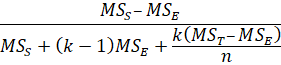
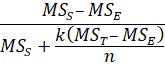
2-way random-effect model: Each subject is assumed to be
assessed by the same group of raters, and raters are assumed to be randomly
sampled from the population. |
||
|
Type of individual scores |
Shrout and
Fleiss Convention |
Computational Formula |
|
Single score from each subject for each trail |
ICC (2,1) |
|
|
Average of k scores from each subject |
ICC (2,k) |
|
|
2-way fixed-effect model: Each subject is assumed to be
assessed by the same group of raters, and raters are only the raters of
interest. |
||
|
Type of individual scores |
Shrout and
Fleiss Convention |
Computational Formula |
|
Single score from each subject for each trail |
ICC (3,1) |
|
|
Average of k scores from each subject |
ICC (3,k) |
|
Standard
Error of Measurement (SEM)
Definition
The SEM is a determination of the amount of variation or
spread in the measurement errors for a test, that it refers to the standard
error in estimating observed scores from true scores. SEM has the same units as
the measurement of interest and is usually used to define confidence intervals.
Calculation
![]()
where ![]() is determined from the ANOVA.
is determined from the ANOVA.
Confidence
intervals of true scores and observed scores
The 95% confidence interval of observed score can be
estimated as:
![]()
Similarly, the 95% confidence interval of true score can be
estimated as:
![]()
where T is the estimated true score calculated as ![]() and
and ![]()
Minimum
Detectable Difference (MDD)
Definition
The MDD is the minimum statistically significant difference
between measurements. For changes in the subject s scores which are at least
greater than or equal to the MDD, 95% of them reflect real difference.
Calculation
The SEM could be used to determine MDD as follows:
![]()
Standard
Error of Prediction (SEP)
The SEP is used in defining the confidence intervals
outside which one could be confident that a retest score reflects a real change
in performance. The SEP and the 95% CI are computed as follows:
![]()
The 95% CI is ![]() ,
where
,
where ![]() is the estimated true score.
is the estimated true score.
Example code in SAS
data A;
call streaminit(123); /* set
random number seed */
do i = 1 to 100;
r1 =
rand("Normal",100,50); /* u ~ U(0,1) */
r2 = r1 +
rand("Normal",10,10);
output;
end;
run;
data test_long;
set A;
array s(2) r:;
do judge = 1 to 2;
y = s(judge);
output;
end;
run;
%macro Icc_sas(ds, response, subject);
ods output OverallANOVA =all;
proc glm data=&ds;
class
&subject;
model
&response=&subject;
run;
data Icc(keep=sb
sw n R R_low R_up);
retain
sb sw n;
set
all end=last;
if
source='Model' then sb=ms;
if
source='Error' then do;sw=ms; n=df; end;
if
last then do;
R=round((sb-sw)/(sb+sw), 0.01);
vR1=((1-R)**2)/2;
vR2=(((1+R)**2)/n +((1-R)*(1+3*R)+4*(R**2))/(n-1));
VR=VR1*VR2;
L=(0.5*log((1+R)/(1-R)))-(1.96*sqrt(VR))/((1+R)*(1-R));
U=(0.5*log((1+R)/(1-R)))+(1.96*sqrt(VR))/((1+R)*(1-R));
R_Low=(exp(2*L)-1)/(exp(2*L)+1);
R_Up=(exp(2*U)-1)/(exp(2*U)+1);
output;
end;
run;
proc
print data=icc noobs split='*';
var
r r_low r_up;
label
r='ICC*' r_low='Lower bound*' r_up='Upper
bound*';
title
'Reliability test: ICC and its confidence limits';
run;
%mend;
%Icc_sas(test_long, response = y, subject
= judge);
proc means data=test_long std;
var y;
run;
data;
icc = 0.44;
SD = 47.9575252;
SEM = SD
* sqrt(1-icc);
SEM_TS = SD * sqrt(icc*(1-icc));
MD = SEM * 1.96 * sqrt(2);
MD_TS = SEM_TS * 1.96 * sqrt(2);
SEP = SD *
sqrt(1-icc);
run;
Example code in R
library(psych)
library(tidyverse)
# Simulate data.
# For the input data, you need a
data frame that has 2 coloumns and n rows.
# This data can be any data - but
repeat reading/measure from the same reader per row
set.seed(1)
n <- 100
r1 <- rnorm(n, mean = 100, sd = 50)
r2 <- r1 + rnorm(n, mean = 10, sd = 10)
data <- tibble(
read1 = r1,
read2 = r2
)
# SEM and MDD function.
## For SEM, you need either ICC(2,1) or ICC(3,1).
get_sem_mdd <- function(data, icc_type){
# Calculate SEM - equation (8).
## Get SD first.
SD <- data %>%
pivot_longer(everything()) %>%
pluck('value') %>%
sd()
## Get ICC.
data_icc <- ICC(data)$results
icc <- data_icc
%>%
filter(
type %in% icc_type
) %>%
pluck('est')
## Calculate SEM
SEM <- SD * sqrt(1-icc)
## SEM_TS equation (11)
SEM_TS <- SD * sqrt(icc*(1-icc))
## MD equation (12)
MD <- SEM * qnorm(0.975) * sqrt(2)
MD_TS <- SEM_TS * qnorm(0.975) * sqrt(2)
## SEP equation (15)
SEP <- SD * sqrt(1-icc)
result <- tibble(
SD,
SEM,
SEM_TS,
MD,
MD_TS,
SEP
)
return(result)
}
get_sem_mdd(data, 'ICC2')
References
1.
Harvill,
L.M. (1991). Standard Error of Measurement. Educational Measurement: Issues and
Practice, 10, 33-41.
2.
Weir
J. P. (2005). Quantifying test-retest reliability using the intraclass
correlation coefficient and the SEM. Journal
of strength and conditioning research, 19(1),
231 240. https://doi.org/10.1519/15184.1
3.
Hopkins
W. G. (2000). Measures of reliability in sports medicine and science. Sports medicine (Auckland, N.Z.), 30(1), 1 15.
https://doi.org/10.2165/00007256-200030010-00001
4.
Duquesne,
S., Alalouni, U., Gr ff,
T., Frische, T., Pieper, S., Egerer,
S., Gergs, R., & Wogram,
J. (2020). Better define beta-optimizing MDD (minimum detectable difference)
when interpreting treatment-related effects of pesticides in semi-field and
field studies. Environmental science
and pollution research international, 27(8),
8814 8821. https://doi.org/10.1007/s11356-020-07761-0